This was definitely the most difficult Jane Street puzzle I have solved so far. You can find solutions to previous Jane Street puzzles I’ve solved here and here.

The Robot Weightlifting World Championship’s final round is about to begin! Three robots, seeded 1, 2, and 3, remain in contention. They take turns from the 3rd seed to the 1st seed publicly declaring exactly how much weight (any nonnegative real number) they will attempt to lift, and no robot can choose exactly the same amount as a previous robot. Once the three weights have been announced, the robots attempt their lifts, and the robot that successfully lifts the most weight is the winner. If all robots fail, they just repeat the same lift amounts until at least one succeeds.

Assume the following:

1) all the robots have the same probability p(w) of successfully lifting a given weight w;

2) p(w) is exactly known by all competitors, continuous, strictly decreasing as the w increases, p(0) = 1, and p(w) -> 0 as w -> infinity; and

3) all competitors want to maximize their chance of winning the RWWC.

If w is the amount of weight the 3rd seed should request, find p(w). Give your answer to an accuracy of six decimal places.

Weights vs probabilities

While trying to model this problem mathematically, notice that the weights are not directly of importance: only $p(w)$ is. $p(w)$ is strictly decreasing and continuous, therefore bijective. It also holds that $w_i < w_j \iff p(w_i) > p(w_j)$. Therefore, we can work directly with the probabilities of succesful lifts, and reason about the ordering of weights from this probabilities. With this simple rework we simplify the problem massively. Let’s denote the probabilities of succesful lifts by $p_1$, $p_2$ and $p_3$. Robot #3 starts the game by choosing $p_3$.

We can make a simulation to get an approximate overview of the problem:

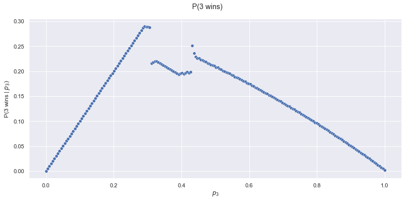
A graph that shows the probability of robot 3 winning versus p3.

In reality, the full range of $p_1, p_2, p_3$ is $(0, 1]$, an infinite amount of points. To simplify this, I chose 400 evenly distributed points on this continuous range (that was the max my computer could handle in a reasonable amount of time). That causes some small artifacts, some lines show some sort of jumping pattern, but we still get a good overview of the game if we ignore these artifacts for now.

Unfortunately, this brute force algorithm is too inefficient to solve the problem to 6 decimal digits of precision. In that case, we would have to choose at least $10^6$ points for all three variables. This algorithm has time complexity $O((10^n)^3) = O(1000^n)$ where n is the required precision. Definitely not quick enough for $n=6$.

We can see that our optimal $p_3$ is somewhere around $0.28$. That value of $p_3$ maximizes the probability of robot 3 winning. That will be our new goal, find the exact $p_3$ that corresponds to the kink at 0.28. Let’s redefine our boundaries on $p_3$ and zoom in:

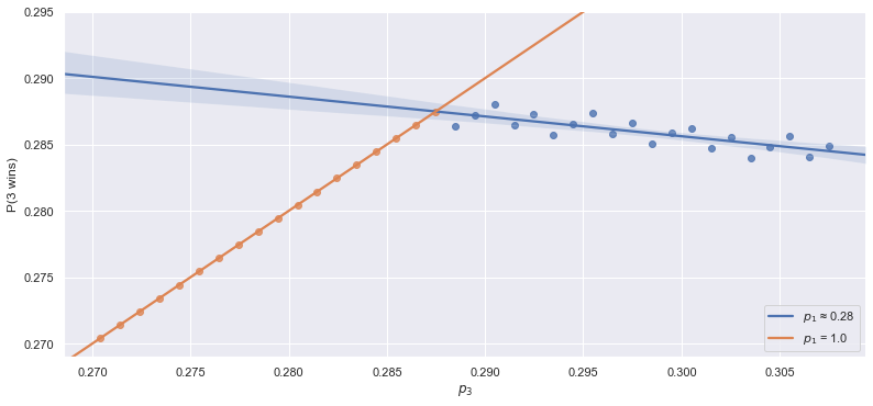
The same graph as above, zoomed in around the maximum of p3

You can clearly see the rounding artifacts in this image. Notice I’ve added colours: orange corresponds to optimal solutions where $p_1 = 1.0$. Consider the following data:

P(2 wins)	$p_1$	$p_2$	$p_3$
0.311602	1.000000	0.436090	0.285464
0.311165	1.000000	0.436090	0.286466
0.310728	1.000000	0.436090	0.287469
0.311596	0.288221	0.441103	0.288471
0.310984	0.288221	0.441103	0.289474
0.310372	0.288221	0.441103	0.290476

Notice the sudden flip of optimal $p_1$ when we increase $p_3$ too much. It is equal to 1.0 at first, but suddenly changes to ~0.28. The kink in the graph seems to correspond with the exact point where the optimal strategy for robot 1 switches from choosing $p_1 = p_3 - \epsilon$ (more on that later) to $p_1 = 1.0$. It makes sense that this optimum point for robot #3 corresponds to a strategy switch of another player: at some point, robot #3 has made $p_3$ so large that it provides robot #1 the opportunity to “undercut” $p_3$ (aka choose a slightly bigger weight than robot #3) and increase his chance of winning.

Layers of argmax

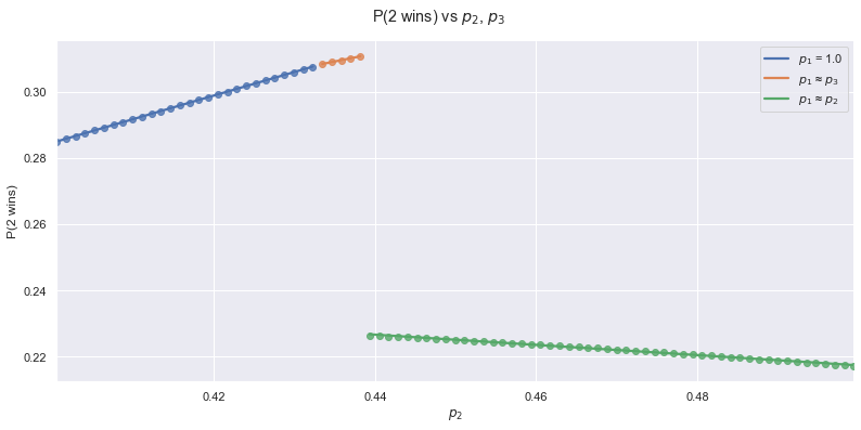
Let’s fix $p_3$ and look at the graph of $p_2$ versus the probability of robot 2 winning (use the slider to change $p_3$!):

$$p_3$$

Notice that across the entire $0.0 < p_3 < 0.31$ range, the optimal $p_2$ corresponds to the rightmost discontinuity. If we zoom in on this discontinuity, we find the following image:

The same graph as above, zoomed in around the maximum of p2

This time, we have three different approximate values of $p_1$: $p_1=p_3 - \epsilon$, $p_1 = p_2 - \epsilon$ or $p_1 = 1.0$. Why these values? Consider the following graph, where we fix both $p_3$ and $p_2$ (use the sliders to change their values!):

$$p_2$$

$$p_3$$

Notice that no matter what values you choose via the sliders, you always have the same values for the discontinuities on the horizontal axis: $p_2$, $p_3$ and $1.0$. Furthermore, a maximum of this graph always corresponds to one of these discontinuities, as the function is increasing. This makes it easy to create a reaction function for robot #1: evaluate the chance of winning for the three possible values of $p_1$ and choose the one with the highest probability of winning. It’s easy to obtain $p_1$ this way, and, most importantly, we get the value of $p_1$ to an arbitrary amount of decimals. This reaction function of robot #1 will be called $R_1(p_2, p_3)$.

Back to robot #2: for a given $p_3$, and now that we know how robot #1 will react to robot #2 and #3, how can we figure out the exact optimal value of $p_2$?

The first binary search

Let’s create the following indicator function:

\[𝟙_2(p_2, p_3) = \begin{cases} 1 & & \mathbb{P}(\text{1 wins} \mid p_1 = p_2 - \epsilon, p_2, p_3) > \mathbb{P}(\text{1 wins} \mid p_1 = p_3 - \epsilon, &p_2, p_3) \\ & \wedge & \mathbb{P}(\text{1 wins} \mid p_1 = p_2 - \epsilon, p_2, p_3) > \mathbb{P}(\text{1 wins} \mid p_1 = 1.0, &p_2, p_3) \\ 0 & & \text{otherwise} \end{cases}\]

It basically checks whether $p_1 = p_2 - \epsilon$ is the optimal value for $p_1$, and that is equivalent to being to the right of the discontinuity we showed above (e.g. is $p_2$ element of the green dots?).

With this indicator function, we can do a binary search on $p_2$. We keep track of a lower and an upper bound (0.27 and 0.29, for example), and we repeatedly check whether the middle of this interval is to the left or to the right of the discontinuity via the indicator function. If we are to the left of the discontinuity, we set the value of the new lower bound equal to the current middle. In the opposite case, we set the new value of the upper bound equal to the current middle. Because we reduce the size of the interval by half each iteration, we can compute $p_2$ to an arbitrary amount of decimal places in very little time. Each additional digit only takes $log_2(10) \approx 3.32$ iterations to compute. We can calculate $p_2$ to 20 decimal places in only 67 iterations! This algorithm provides us with the reaction function of robot #2: $R_2(p_3)$.

The second binary search

Back to the main question: what value of $p_3$ maximizes the probability of robot #3 winning?

We already found $R_1$ and $R_2$. Therefore we have all we need to create a function that returns the maximum probability of 3 winning given some $p_3$:

\[f(p_3) = \mathbb{P}(\text{3 wins} \mid p_1 = R_1(p_2, p_3), p_2 = R_2(p_3), p_3)\]

I used a trick to check whether $f$ is increasing or decreasing at some $p_3$:

\[𝟙_3(p_3) = \begin{cases} 1 & f(p_3 + \epsilon) - f(p_3) < 0 \\ 0 & \text{otherwise} \end{cases}\]

By incrementing $p_3$ by a small amount ($\epsilon$) and checking the influence of this change on f, we can define an indicator function that checks whether we’re to the left or right of the peak. We apply the same binary search algorithm as described above to this function to find the optimal value to six decimal places: $p_3 = 0.286833$.

Note that $f$ actually depends on a binary search, and we use it within the indicator function of another binary search. This makes the runtime of this algorithm $O(log^2(n))$ where n is the precision in decimal digits. A time complexity I have never encountered before!

My code can be found here.

Analytic solution

I made a lot of assumptions and educated guesses during my initial solve of this problem. The fact that the maximum corresponded exactly to the kink at $p_3 \approx 0.288$, for example. My solution was the result of a lot of trial and error, and a lot of simulations to test my hypotheses. It would be a lot more elegant to solve this problem analytically. The Bellman equation can be used to solve problems with optimal substructure, which this problem seems to belong to. I might revisit this problem in the future and try to solve it that way, as I have not figured out how that method exactly works yet!