A guide to backtracking (w/ Jane Street's December 2020 challenge)

Backtracking is an important concept in computer science and can be used in many different applications. There are many guides on the internet where backtracking is explained with relatively simple problems (n-queens, sudoku, etc.). In this a more challenging problem will be considered, and the intuition you might develop solving it.

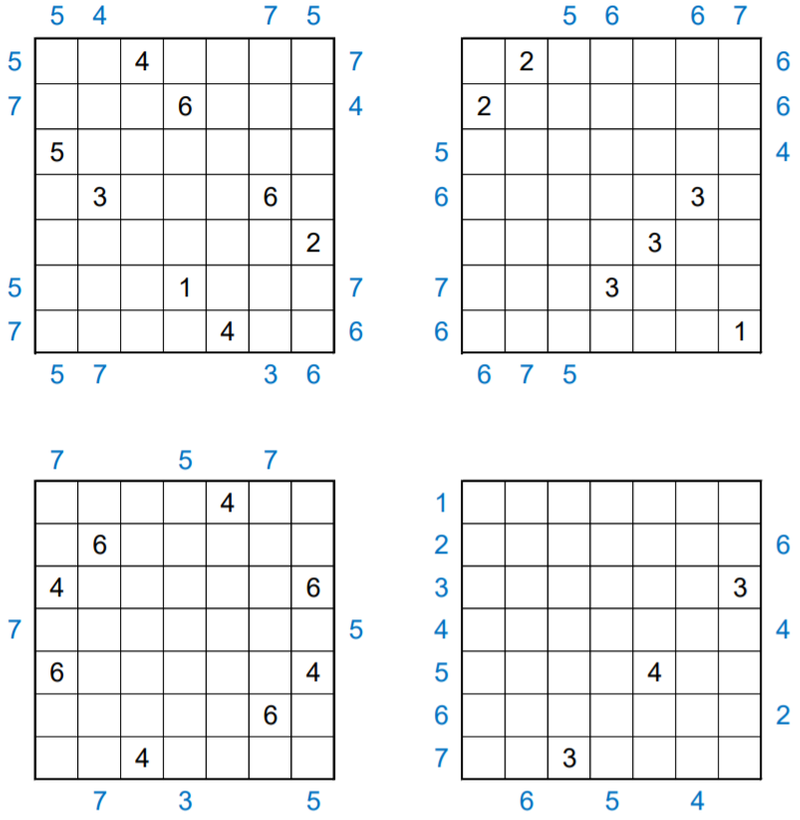
We will look at Jane Street’s December 2020 challenge (Twenty Four Seven 2-by-2 #2):

Each of the grids below is incomplete. Place numbers in some of the empty cells so that in total each grid’s interior contains one 1, two 2’s, etc., up to seven 7’s. Furthermore, each row and column within each grid must contain exactly 4 numbers which sum to 20. Finally, the numbered cells must form a connected region, but every 2-by-2 subsquare in the completed grid must contain at least one empty cell.

Some numbers have been placed inside each grid. Additionally, some blue numbers have been placed outside of the grids. These blue numbers indicate the first value seen in the corresponding row or column when looking into the grid from that location.

Once each of the grids is complete, create a 7-by-7 grid by “adding” the four grids’ interiors together (as if they were 7-by-7 matrices). The answer to this month’s puzzle is the sum of the squares of the values in this final grid.

Some information about backtracking

Generally, backtracking is used when you want to consider all possible solutions to a problem. Fundamentally, backtracking is a variant of path finding in a more abstract space: the space of states and actions.

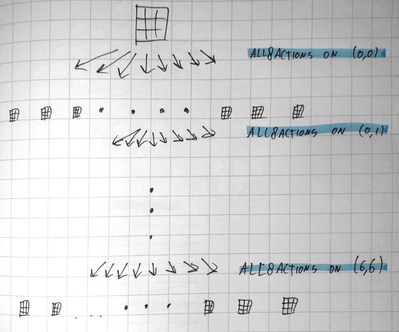
Consider the game as a graph. Each “game state” is a vertex, and each “action” you take is an edge. There are many possible actions. In this instance, we define an action as picking a not yet considered square and choosing to leave it empty or to fill in a number in range 1 through 7.

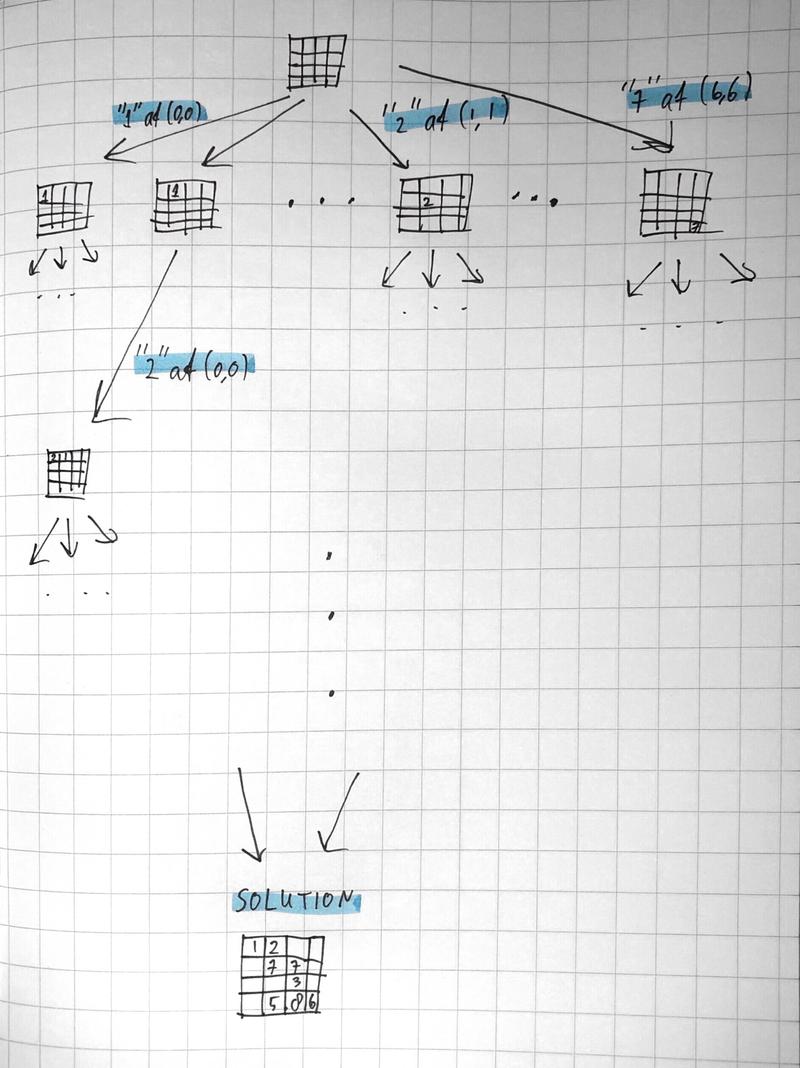
Let’s consider the graph you could make if you start with an empty grid. With an empty grid, there are 49 squares where you can do an action, with 8 possible actions per square (empty or 1-7). After we’ve placed the first number, there are 48 squares left with 8 actions per square, et cetera.

This implies that we end up with \((49\times8)\times(48\times8)\times \dots \times (2\times 8) \times (1 \times 8) = 49! \times 8^{49} \approx 1.08 \times 10^{107}\) final game states.

How big is this number? Imagine a modern desktop computer for every atom in the visible universe. Even if you cluster them into one big supercomputer, brute force computation would still take slightly longer than the age of the universe. That’s where backtracking comes in. The key to backtracking is to cut off a branches of this game tree as quickly as possible:

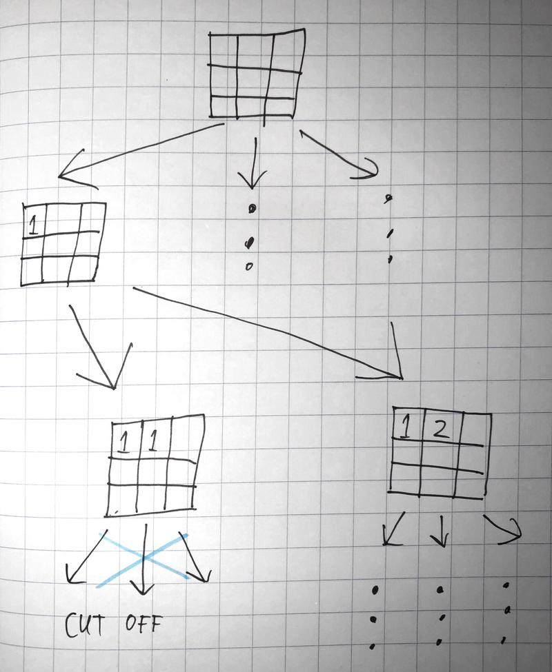
The solution should contain one 1, two 2’s, …, and seven 7’s. As soon as we notice that we have used number 1 two times, we can stop further search from this game state, because we’ll never arrive at the solution anyways. By cutting off the tree this early during the search, we save a massive amount of computation.

There are several observations you should consider when backtracking:

Key observation #1: pruning in the beginning has more effect than pruning at the end

The number of possible states rises exponentially. By cutting off the tree at the beginning you can reduce computation time by a lot. Some constraints are better at cutting off computation early than others. The rule that states that you can only use one 1, for example, already starts cutting off branches at move #2. In contrast, the constraint that all numbers should form one big connected island is less useful at the beginning of the search. There might be multiple disconnected islands at the beginning that converge later on.

Key observation #2: more constraints make computation faster, not slower

This might sound unintuitive. For humans, more rules usually make games more complex, but for computers more rules allow more tree pruning which reduces computation time.

With these observations, we can start optimizing our tree search:

Optimization #1: fix the order of actions

Consider the following two situations:

Situation A:

1. place 2 at (0, 0)
2. place 5 at (0, 1)

Situation B:

1. place 5 at (0, 1)
2. place 2 at (0, 0)

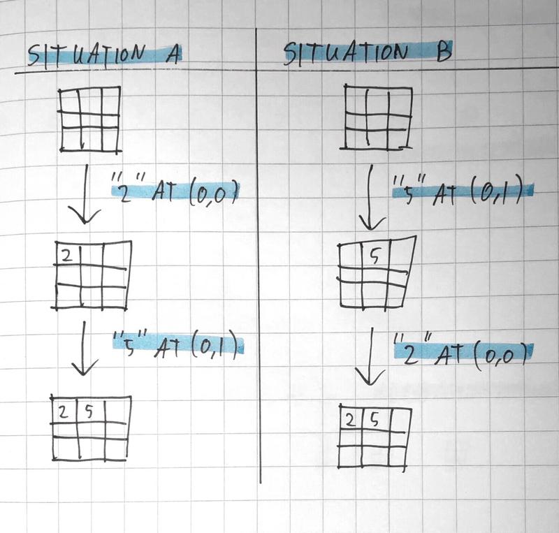
You might notice that both of these situations lead to the same exact puzzle state. If you’ve already ruled out that situation A will never lead to a valid solution, any tree expansion from situation B will be redundant. This means that a naive expansion of the whole tree will lead to an enormous amount of redundant computation: every possible game final game state will be in the expanded tree \(49! \approx 6.08 \times 10^{68}\) times! There is an easy way to fix this: if we visit all coordinates in a fixed order, we can be certain that any state in the tree is unique. With this measure in place, we achieve a massive 608 novemdecillion times speedup.

Optimization #2: use “derivative” weak rules

Consider the following state:

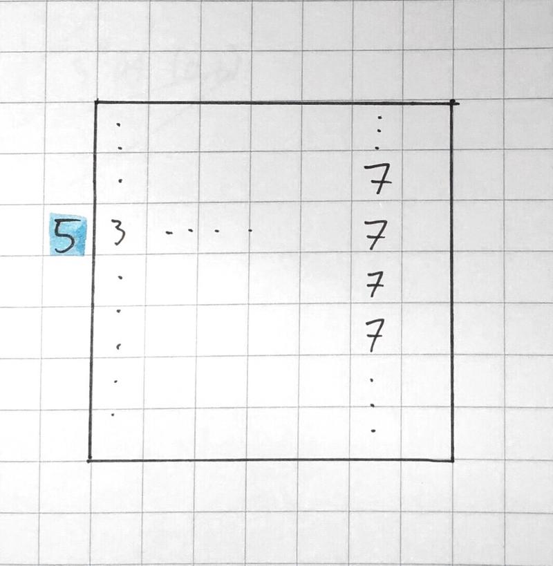
Consider column 6. The sum of that row so far is a 28. Because this sum can never get smaller, we know that this state is invalid. Mind that this is not one of the original constraints. This is a derivative rule of the constraint “the sum of each column is 20”. We can do something similar with row 3: even though that row is not filled yet, we can deduce that this row will never satisfy the constraint that the leftmost number should be a 5.

Similar derivative rules can be derived from the other constraints. Consider the following constraint: “all numbers should form one connected component”. This is a constraint you can only use relatively late in the game: there might be multiple disconnected islands in the beginning that only start to converge later on. However, we can still take advantage of this rule by creating our own “derivative rule”: never block off an island with empty squares. This rule can be enforced more easily at the beginning of the tree, and thus is more valuable when you’re trying to do backtracking.

bool checkColumnWeak(int j) {
    return columnPieces[j] <= 4 && columnSum[j] <= 20
}

// ...

bool checkWVWeak() {
    for (int i = 0; i < 7; i++) {
        if (wv[i] == -1) continue;
        for (int j = 0; j < 7; j++) {
            if (grid[i][j] == 0) continue;
            if (grid[i][j] >= 1 && grid[i][j] != wv[i]) return false;
            break;
        }
    }
    return true;
}
// ... similar functions for north view, east view and south view.

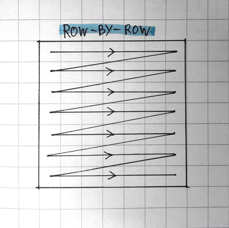
Optimization #3: change the order of actions

There are multiple ways to visit all coordinates one-by-one. The most straightforward way would be row-by-row:

There are also other possible orders in which you can consider squares. Consider a spiral, for example:

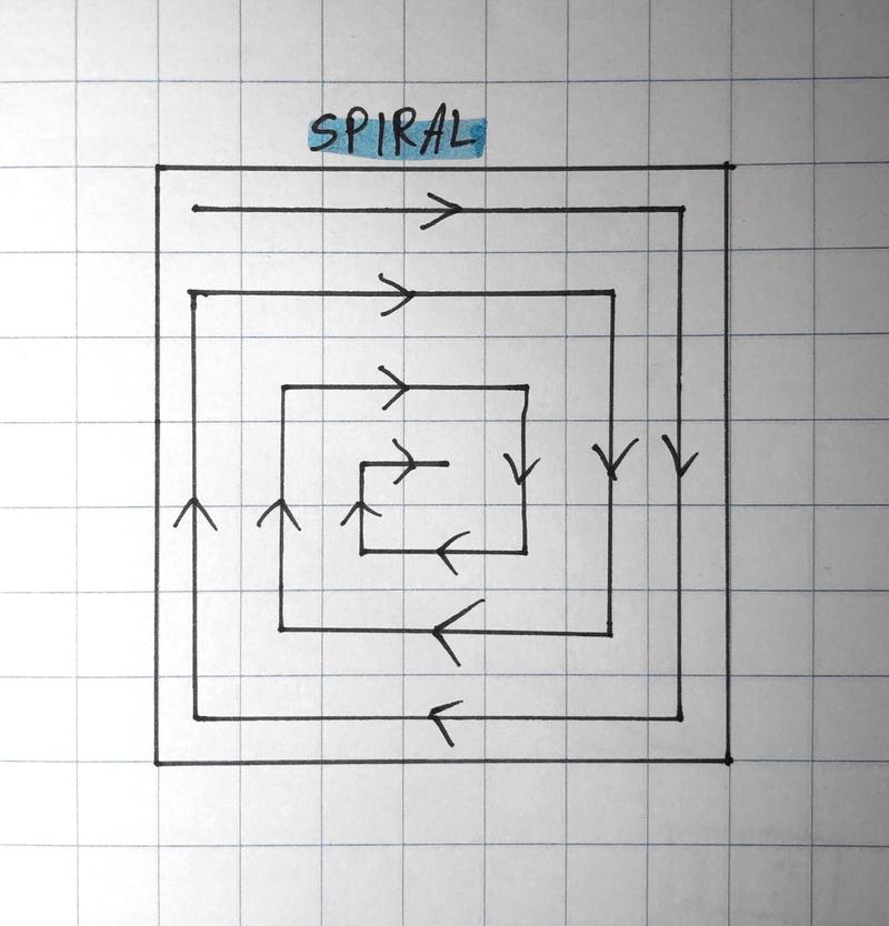
This has two big advantages over the row-by-row order:

1. You can consider whole rows and whole columns earlier. After 7 squares, you can strongly check row #1. 6 squares further, and you can consider column #7, etc. With the row-by-row order you can only consider whole rows every 7 squares, and you can only start checking whole columns all the way at the end of the tree (when you start filling the last row).
2. By tracing along the edge in a spiral, you can start using the side views earlier on in your computation. When you use the row-by-row order, you can only start using the south view when you start filling the last row, for example.

Formulas to calculate which coordinate follows in a spiral exist, though it’s easier and more efficient to just compute a table at the beginning:

pair<int, int> nextCoordinate[7][7];
bool isTurn[7][7];

void initCoordinateOrder() {
    int i = 3, j = 3;
    int di = 0, dj = -1;
    int maxi = 3, mini = 3, maxj = 3, minj = 3;
    for (int k = 0; k < 48; k++) {
        nextCoordinate[i+di][j+dj] = make_pair(i, j);
        i += di;
        j += dj;
        if (i > maxi) {
            maxi = i;
            int buffer = dj;
            dj = di;
            di = -buffer;
            isTurn[i][j] = true;
        }
        if (i < mini) {
            mini = i;
            int buffer = dj;
            dj = di;
            di = -buffer;
            isTurn[i][j] = true;
        }
        if (j > maxj) {
            maxj = j;
            int buffer = dj;
            dj = di;
            di = -buffer;
            isTurn[i][j] = true;
        }
        if (j < minj) {
            minj = j;
            int buffer = dj;
            dj = di;
            di = -buffer;
            isTurn[i][j] = true;
        }
    }
    nextCoordinate[3][3] = make_pair(3, 3);
}

Optimization #4: check connectedness every once in a while

To check connectedness between islands, we do a flood fill across the entire grid every once in a while. This traversal of the whole grid is relatively expensive compared to the other constraint checks we’ve made so far. It happens to be faster to do this check every once in a while than to do it on every action.

There are alternatives to doing a whole flood fill to check connectedness. You could use a disjoint-set structure for example to keep track of which components are connected to which other components, for example. For small grids such as this one the speed difference with flood fill would probably be marginal, but especially for larger grids a disjoint-set structure would yield increasingly higher speed ups (floodfill takes \(O(n^2)\) while disjoint-set takes \(O(log(n))\)).

Conclusion

You can look at my implementation here. With all of these optimizations in place, solving all 4 grids takes less than 1 second on an Intel Core i5-6300HQ. I would like to thank Jane Street for their monthly challenges, this was an interesting problem with endless possibilities to speed up computation.